code_base

library(tidyverse)

Warning: package 'tidyverse' was built under R version 4.3.2

Warning: package 'ggplot2' was built under R version 4.3.3

Warning: package 'tidyr' was built under R version 4.3.2

Warning: package 'readr' was built under R version 4.3.2

Warning: package 'dplyr' was built under R version 4.3.2

Warning: package 'stringr' was built under R version 4.3.2

Warning: package 'lubridate' was built under R version 4.3.2

── Attaching core tidyverse packages ──────────────────────── tidyverse 2.0.0 ──
✔ dplyr     1.1.4     ✔ readr     2.1.5
✔ forcats   1.0.0     ✔ stringr   1.5.1
✔ ggplot2   3.5.1     ✔ tibble    3.2.1
✔ lubridate 1.9.3     ✔ tidyr     1.3.1
✔ purrr     1.0.2     
── Conflicts ────────────────────────────────────────── tidyverse_conflicts() ──
✖ dplyr::filter() masks stats::filter()
✖ dplyr::lag()    masks stats::lag()
ℹ Use the conflicted package (<http://conflicted.r-lib.org/>) to force all conflicts to become errors

library(dplyr)
library(RColorBrewer)
library(stringr)

Code Base

nobel_data <- read.csv("../data/nobel_laureates_data.csv")
head(nobel_data)

  year   category
1 2023   medicine
2 2023  economics
3 2023      peace
4 2023 literature
5 2023  chemistry
6 2023  chemistry
                                                                                                                               motivation
1 for their discoveries concerning nucleoside base modifications that enabled the development of effective mRNA vaccines against COVID-19
2                                                                  for having advanced our understanding of womens labour market outcomes
3                         for her fight against the oppression of women in Iran and her fight to promote human rights and freedom for all
4                                                                    for his innovative plays and prose which give voice to the unsayable
5                                                                                         for the discovery and synthesis of quantum dots
6                                                                                         for the discovery and synthesis of quantum dots
  prizeShare laureateID         fullName gender       born bornCountry
1          2       1024   Katalin Kariko female 17-01-1955     Hungary
2          1       1034   Claudia Goldin female 1946-00-00         USA
3          1       1033 Narges Mohammadi female 21-04-1972        Iran
4          1       1032        Jon Fosse   male 29-09-1959      Norway
5          3       1031    Alexei Ekimov   male 1945-00-00      Russia
6          3       1030       Louis Brus   male 1943-00-00         USA
      bornCity       died diedCountry diedCity             organizationName
1      Szolnok 0000-00-00                                 Szeged University
2  New York NY 0000-00-00                                Harvard University
3       Zanjan 0000-00-00                                                  
4    Haugesund 0000-00-00                                                  
5              0000-00-00                      Nanocrystals Technology Inc.
6 Cleveland OH 0000-00-00                               Columbia University
  organizationCountry organizationCity
1             Hungary           Szeged
2                 USA     Cambridge MA
3                                     
4                                     
5                 USA      New York NY
6                 USA      New York NY

nobel_data <- nobel_data %>% filter(gender != "org") %>% distinct(fullName, .keep_all = TRUE)

# Quick look
nobel_data$category %>% factor() %>% levels()

[1] "chemistry"  "economics"  "literature" "medicine"   "peace"     
[6] "physics"   

nobel_data$gender %>% table()

.
female   male 
    64    901 

nobel_data$year <- nobel_data$year %>% as.numeric()
nobel_data %>% select(bornCountry) %>% table()

bornCountry
                         Algeria                        Argentina 
                               2                                4 
                       Australia                          Austria 
                              10                               19 
                      Azerbaijan                       Bangladesh 
                               1                                1 
                         Belarus                          Belgium 
                               4                                9 
          Bosnia and Herzegovina                           Brazil 
                               2                                1 
                        Bulgaria                           Canada 
                               1                               21 
                           Chile                            China 
                               2                               12 
                        Colombia                       Costa Rica 
                               2                                1 
                         Croatia                           Cyprus 
                               1                                1 
                  Czech Republic Democratic Republic of the Congo 
                               6                                1 
                         Denmark                       East Timor 
                              12                                2 
                           Egypt                         Ethiopia 
                               6                                1 
         Faroe Islands (Denmark)                          Finland 
                               1                                5 
                          France                          Germany 
                              61                               84 
                           Ghana                           Greece 
                               1                                1 
               Guadeloupe Island                        Guatemala 
                               1                                2 
                         Hungary                          Iceland 
                              11                                1 
                           India                        Indonesia 
                               9                                1 
                            Iran                             Iraq 
                               3                                1 
                         Ireland                           Israel 
                               5                                6 
                           Italy                            Japan 
                              20                               28 
                           Kenya                           Latvia 
                               1                                1 
                         Lebanon                          Liberia 
                               1                                2 
                       Lithuania                       Luxembourg 
                               3                                2 
                      Madagascar                           Mexico 
                               1                                3 
                         Morocco                          Myanmar 
                               1                                1 
                     Netherlands                      New Zealand 
                               1                                3 
                         Nigeria                  North Macedonia 
                               1                                1 
                Northern Ireland                           Norway 
                               5                               13 
                        Pakistan                             Peru 
                               3                                1 
                     Philippines                           Poland 
                               1                               28 
                        Portugal                          Romania 
                               2                                4 
                          Russia                      Saint Lucia 
                              29                                2 
                        Scotland                         Slovakia 
                              11                                1 
                        Slovenia                     South Africa 
                               1                                9 
                     South Korea                            Spain 
                               2                                7 
                          Sweden                      Switzerland 
                              30                               19 
                          Taiwan                         Tanzania 
                               1                                1 
                 the Netherlands              Trinidad and Tobago 
                              18                                1 
                         Tunisia                           Turkey 
                               1                                2 
                         Turkiye                          Ukraine 
                               1                                5 
                  United Kingdom                              USA 
                              89                              289 
                       Venezuela                          Vietnam 
                               1                                1 
                           Yemen                         Zimbabwe 
                               1                                1 

(17/64)

[1] 0.265625

(283/965)

[1] 0.2932642

## Too many levels
#nobel_data$year %>% factor() %>% levels()
n#obel_data$bornCountry %>% factor() %>% levels()

function () 
{
    peek_mask()$get_current_group_size()
}
<bytecode: 0x000001201d2f4c90>
<environment: namespace:dplyr>

Alright

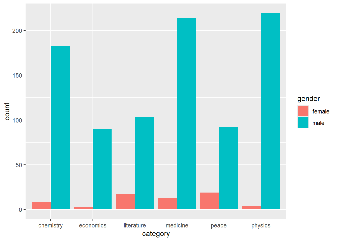
So the plan is to do vertical slices by category and compare whether the gender distribution across them is the same or different. I think thats a decent project goal and then I can do visualizations with the trends over time.

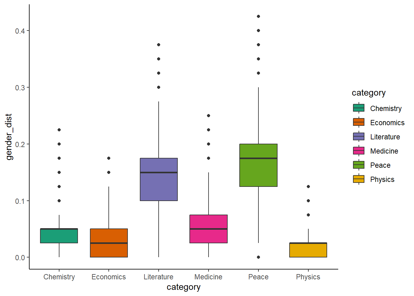
I’ll use a bit of bootstrapping in order to get this to work

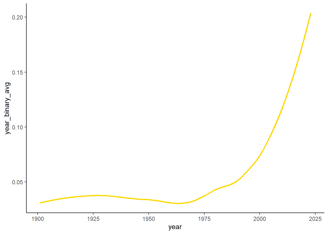
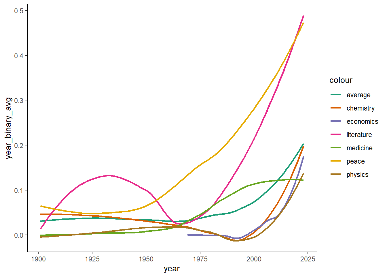
## Setting female/male table to binary
nobel_gender <- nobel_data %>% select(gender)
nobel_gender[nobel_gender$gender == "male",1] <- 0
nobel_gender[nobel_gender$gender == "female",1] <- 1

nobel_data$gender_binary <- nobel_gender[,1] %>% as.numeric()
nobel_data$year_char <- nobel_data$year %>% as.character()

## Year average
year_binary_avg <- aggregate(nobel_data$gender_binary, list(nobel_data$year_char), FUN = mean) 
colnames(year_binary_avg) <- c("year_char","year_binary_avg")

nobel_data <- left_join(nobel_data,year_binary_avg, by = "year_char")

## year average by category
year_cat_binary_avg <- aggregate(nobel_data$gender_binary, list(nobel_data$year_char,nobel_data$category), FUN = mean) 
colnames(year_cat_binary_avg) <- c("year_char","category","year_cat_binary_avg")

nobel_data <- left_join(nobel_data,year_cat_binary_avg, by = c("year_char","category"))

count_nobel <- nobel_data %>% count(category,gender)
female_count <- count_nobel %>% filter(gender == "female")
female_count2 <- female_count$n
male_count <- count_nobel %>% filter(gender == "male")
male_count2 <- male_count$n

count_table <- rbind(female_count2,male_count2) %>% as.data.frame()
colnames(count_table) = female_count$category

model <- chisq.test(count_table)
model

    Pearson's Chi-squared test

data:  count_table
X-squared = 43.023, df = 5, p-value = 3.655e-08

ggplot(data = nobel_data, aes(x = category,fill = gender)) + geom_bar(position = "dodge")

ggplot(data = nobel_data,aes(x = year, y = year_binary_avg)) + geom_smooth(color = "gold",se = FALSE) + 
  theme_classic()

`geom_smooth()` using method = 'loess' and formula = 'y ~ x'

ggplot(data = nobel_data) + 
  geom_smooth(aes(x = year,y = year_binary_avg,color = "average"),se= FALSE) + 
  geom_smooth(aes(x = year,y = year_cat_binary_avg, color = category), se = FALSE) +
  scale_color_brewer(palette = "Dark2") +
  theme_classic()

`geom_smooth()` using method = 'loess' and formula = 'y ~ x'
`geom_smooth()` using method = 'loess' and formula = 'y ~ x'

### creating bootstraps

# initializing vectors
chem_boot <- c()
econ_boot <- c()
lite_boot <- c()
medi_boot <- c()
peac_boot <- c()
phys_boot <- c()

chem_data <- nobel_data %>% filter(category == "chemistry") %>% select(gender_binary)
econ_data <- nobel_data %>% filter(category == "economics") %>% select(gender_binary)
lite_data <- nobel_data %>% filter(category == "literature") %>% select(gender_binary)
medi_data <- nobel_data %>% filter(category == "medicine") %>% select(gender_binary)
peac_data <- nobel_data %>% filter(category == "peace") %>% select(gender_binary)
phys_data <- nobel_data %>% filter(category == "physics") %>% select(gender_binary)

sample_take_mean_return <- function(data,n){
  data_sample <- sample(data[,1],size = n, replace = TRUE)
  mean_sample <- mean(data_sample)
  return(mean_sample)
}

n <- 40


for(i in 1:10000){
  n <- 40
  chem_boot <- c(chem_boot,sample_take_mean_return(chem_data,n))
  econ_boot <- c(econ_boot,sample_take_mean_return(econ_data,n))
  lite_boot <- c(lite_boot,sample_take_mean_return(lite_data,n))
  medi_boot <- c(medi_boot,sample_take_mean_return(medi_data,n))
  peac_boot <- c(peac_boot,sample_take_mean_return(peac_data,n))
  phys_boot <- c(phys_boot,sample_take_mean_return(phys_data,n))
  
}


chem_boot_df <- chem_boot %>% data.frame()
chem_boot_df$category <- "Chemistry"

econ_boot_df <- econ_boot %>% data.frame()
econ_boot_df$category <- "Economics"

lite_boot_df <- lite_boot %>% data.frame()
lite_boot_df$category <- "Literature"

medi_boot_df <- medi_boot %>% data.frame()
medi_boot_df$category <- "Medicine"

peac_boot_df <- peac_boot %>% data.frame()
peac_boot_df$category <- "Peace"

phys_boot_df <- phys_boot %>% data.frame()
phys_boot_df$category <- "Physics"

boot_df <- rbind(chem_boot_df,econ_boot_df,lite_boot_df,medi_boot_df,peac_boot_df,phys_boot_df)
colnames(boot_df)[1] <- "gender_dist"

library(multcompView)

Warning: package 'multcompView' was built under R version 4.3.3

anova <- aov(data = boot_df, gender_dist ~ category)
summary(anova)

               Df Sum Sq Mean Sq F value Pr(>F)    
category        5  200.8   40.15   23901 <2e-16 ***
Residuals   59994  100.8    0.00                   
---
Signif. codes:  0 '***' 0.001 '**' 0.01 '*' 0.05 '.' 0.1 ' ' 1

#tukey <- TukeyHSD(x = anova, 'category',conf.level = .95)

ggplot(data = boot_df, aes(x = category,y = gender_dist,fill = category)) +
  geom_boxplot() + 
  theme_classic()+
  scale_fill_brewer(palette = "Dark2")

for(i in 1:nrow(nobel_data)){
  col <- nobel_data %>% select(born)
  in_check <- grepl("-",col[i,1])
  if(in_check == TRUE){
    row <- str_split(col[i,1],pattern = "-")
  } else{
    row <- str_split(col[i,1],pattern = "/")
  }
  if(i == 1){
    df <- row[[1]] %>% t() %>% as.data.frame()
  } else{
    df <- rbind(df,row[[1]])
  }
}

year_born_accum <- c()
for(i in 1:nrow(df)){
  bit <- df[i,]
  for(g in 1:ncol(bit)){
    if(nchar(bit[1,g])==4){
      year_born_accum <- c(year_born_accum,bit[1,g])
    } 
  }
}

nobel_data$year_born <- year_born_accum %>% as.numeric()
nobel_data$year <- nobel_data$year %>% as.numeric()
nobel_data <- nobel_data %>% mutate(age_of_award = year - year_born)

gender_data2 <- nobel_data %>% filter(gender != "org")
summary(gender_data2$age_of_award)

gender_data2 %>% filter(age_of_award == 97) 

model <- lm(data = gender_data2,gender_binary ~ year + category + prizeShare + age_of_award + year*category)
summary(model)